| System | \mathcal{P} | {\mathcal{P} \! / \!\! \sim_\mathrm{B}} | \mathrel{\smash{›\!\!\frac{\scriptstyle{\;\enspace\;}}{}\!\!›}}_{\blacktriangle} | time (s) | {\mathcal{P} \! / \!\! \sim_\mathrm{E}} | {\mathcal{P} \! / \!\! \sim_\mathrm{T}} | {\mathcal{P} \! / \!\! \sim_\mathrm{1S}} |
|---|---|---|---|---|---|---|---|
peterson |
36 | 31 | 4,602 | 0.05 | 10 | 30 | 30 |
vasy_0_1 |
289 | 9 | 566 | 0.01 | 3 | 9 | 9 |
cwi_1_2 |
1,952 | 1,132 | 22,707,217 | 195.39 | 11 | 1,132 | 1,132 |
vasy_1_4 |
1,183 | 28 | 1,000 | 0.01 | 8 | 28 | 28 |
cwi_3_14 |
3,996 | 62 | 18,350 | 0.15 | 3 | 62 | 62 |
vasy_5_9 |
5,486 | 145 | 2,988 | 0.03 | 109 | 145 | 145 |
vasy_8_24 |
8,879 | 416 | 145,965 | 1.44 | 177 | 416 | 416 |
vasy_8_38 |
8,921 | 219 | 14,958 | 0.16 | 115 | 219 | 219 |
vasy_10_56 |
10,849 | 2,112 | 6,012,676 | 97.89 | 14 | 2,112 | 2,112 |
vasy_18_73 |
18,746 | 4,087 | - | - | - | - | - |
vasy_25_25 |
25,217 | 25,217 | 0 | 0.24 | 25,217 | 25,217 | 25,217 |
8 Implementations
All the nice theory of preceding chapters also works in practice. This chapter revisits the core parts of the thesis by discussing how they tie together in a tool implementation.
The tool, equiv.io, will be presented in Section 8.1. We demonstrate its use through the example of Peterson’s mutex. Section 8.2 shows that the game approach lends itself to many things: To explain equivalence notions in a computer game, to extend existing tools, and to parallelize equivalence checking through GPUs. In Section 8.3, we compare our implementations to similar tools in the lineage of the “Concurrency Workbench” (Cleaveland et al., 1990).
8.1 Prototype: equiv.io
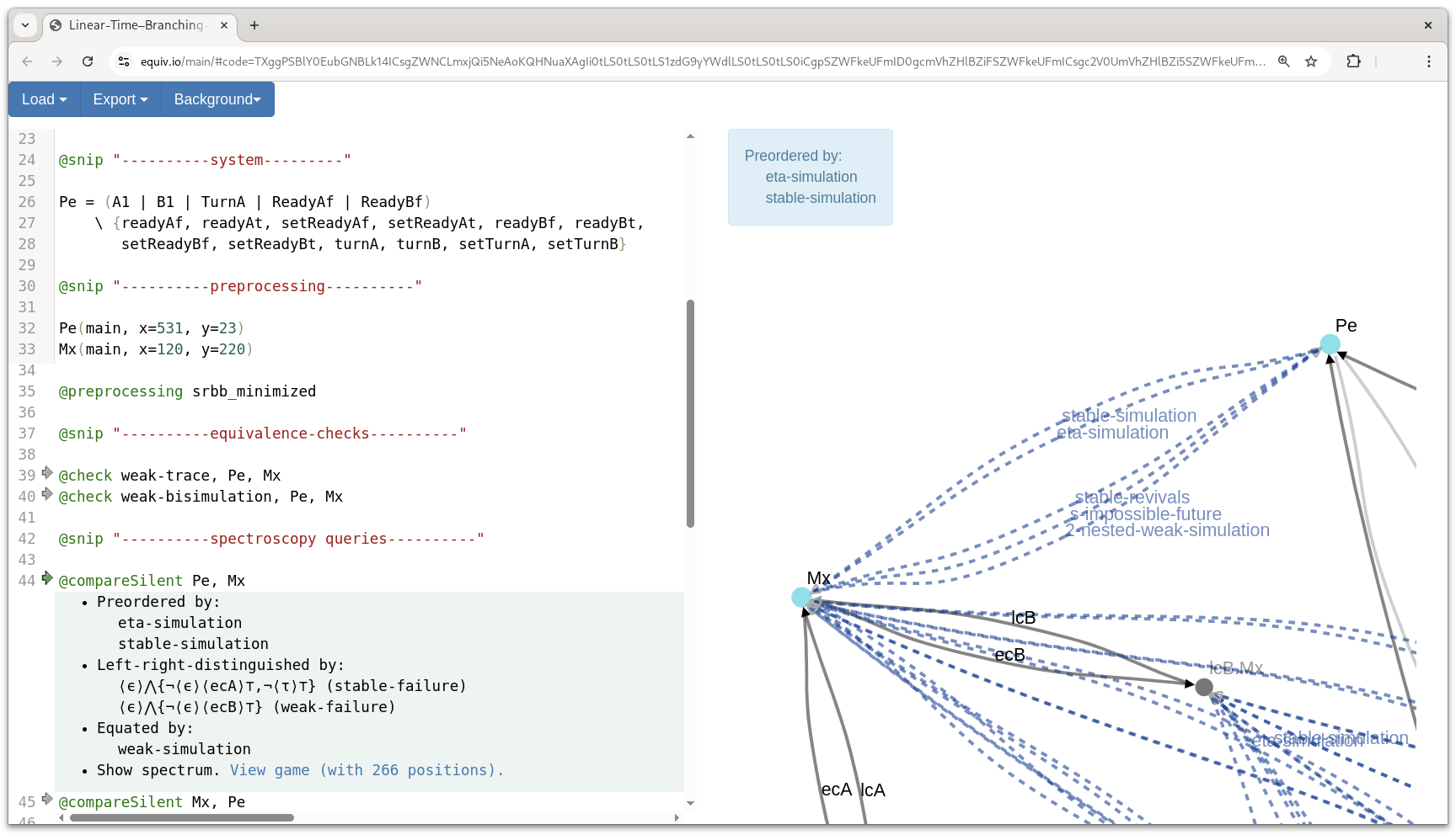
The “Linear-time–branching-time spectroscope” at equiv.io is a small web tool to check equivalence and preorder relations on CCS processes. Figure 8.1 shows a screenshot. In this section, we will discuss its usage (Section 8.1.1), apply it to the Peterson example (Section 8.1.2), examine the tool structure (Section 8.1.3), and benchmark its backend (Section 8.1.4).
8.1.1 Usage
The standard workflow of equiv.io is to specify processes in CCS and then compare them with respect to equivalence spectra. This is mainly achieved by writing text into the source editor on the left. The specific order of definitions, queries, and declarations in the source generally makes no difference.
Process syntax. CCS processes are written according to the grammar in Definition 2.2, with the concrete syntax for subterms following Table 8.1.
| Construct | Tool syntax | \textsf{CCS} |
|---|---|---|
| Input prefix | a.P |
\mathsf{a}\ldotp\! P |
| Output prefix | a!P |
\overline{\mathsf{a}}\ldotp\! P |
| Internal action | tau.P |
\tau\ldotp\! P |
| Null process | 0 |
\mathbf{0} |
| Recursion | P_Name |
\mathsf{P_{Name}} |
| Choice | P1 + P2 |
P_1 +P_2 |
| Parallel | P1 | P2 |
P_1 \mid P_2 |
| Restriction | P \ {a1, a2} |
P \mathbin{\backslash}\{\mathsf{a_1}, \mathsf{a_2}\} |
Literals for actions and process names combine Latin letters, numbers, and underscores in the usual way.
Top-level process definitions are written X = P, expressing that \mathcal V(\mathsf{X}) \mathrel{≔}P in the semantics (Definition 2.3). The right-hand pane shows the resulting transition system and output (cf. Figure 8.1).
The syntax tree can be clarified by parentheses “(...)”. Otherwise, the parser reads prefix “a._” with highest operator precedence, then restriction “_ \ {_}”, then choice “+” and parallel “|” at equal level. In case of ambiguity, it assumes parenthesization from the right.
Equivalence queries. Queries for the behavioral equivalences between states are formulated in the source editor as well and are started by clicking on the arrows that pop up in the gutter. Output will appear right below the query in the editor. The standard queries are:
@compare P1, P2– Perform a spectroscopy onP1andP2with respect to the strong spectrum using the game of Chapter 5. The output will have four items, relative to the strong spectrum.- The strongest preorders to relate
P1toP2; - Cheapest formulas to distinguish
P1fromP2(and the smallest observation language they are part of); - The list of finest equivalences to equate
P1andP2. - A visualization of the result on the whole spectrum. Moreover, there will be a link to a https://edotor.net/-visualization of the game graph used to obtain the result. The naming of notions in the output follows Table 8.2.
- The strongest preorders to relate
@compareSilent P1, P2– Perform a spectroscopy onP1andP2with respect to the weak spectrum, treating silent steps along the lines of Chapter 7. The output is analogous to@compare.@check equivalence-name, P1, P2– Checks for (mutual) preordering betweenP1andP2with respect to individual notionequivalence-name. The name of the notion to be checked must be one of the ones in Table 8.2.
| Strong variant | Weak variants | Stable/stability-resp. variants |
|---|---|---|
enabledness |
weak-enabledness |
|
trace |
weak-trace |
|
failure |
weak-failure |
stable-failure |
revivals |
stable-revivals |
|
readiness |
weak-readiness |
stable-readiness |
failure-trace |
stable-failure-trace |
|
ready-trace |
stable-ready-trace |
|
impossible-future |
weak-impossible-future |
s-impossible-future |
possible-future |
weak-possible-future |
|
simulation |
weak-simulation eta-simulation |
stable-simulation |
ready-simulation |
weak-ready-simulation |
s-ready-simulation |
2-nested-simulation |
2-nested-weak-simulation |
|
bisimulation |
contrasimulationweak-bisimulationdelay-bisimulationeta-bisimulationbranching-bisimulation |
stable-bisimulationsr-delay-bisimulationsr-branching-bisimulation |
Interacting with the output. Each output item can be clicked. The transition system view then displays the preorders, equivalences, and distinctions that have been found between states.
States in the transition system may be dragged to change their position. The layout information is persisted in the source, as described in the next list.
Layout and preprocessing. The source can also contain layout information and prescribe some preprocessing for processes.
P(main)– Highlight processPin the transition system and prune other sub-processes (unless they are reached fromP). Multiple processes may be declared to bemain.P(x=100, y=100)– Annotate processPto be displayed at certain coordinates."0"(x=100, y=200)– The annotations may also refer to subprocesses The CCS expressions are wrapped in"...". They must be verbatim the string representation the tool uses for the normalized process.@preprocessing method1, method2...– Apply preprocessing to the transition system after translation of the CCS term (that is, before presentation and queries happen). This will affect the whole transition system, but tries to preserve processes that have been marked asmain. The order of processing steps can make a difference. The supported methods are:weakness_saturated– Replace the transition relation with weak transitions. In effect, there will be a transition whenever the original system allows \mathrel{\twoheadrightarrow}\xrightarrow{\smash{\raisebox{-2pt}{$\scriptstyle{(\alpha)}$}}}\mathrel{\twoheadrightarrow}.tauloop_compressed_marked– Collapse states on \tau-loops and mark them with a \delta. (This follows the thought of how to make equivalence queries divergence-respecting from Section 7.3.3.)bisim_minimized– Merge states that are strongly bisimilar.srbb_minimized– Merge states that are stability-respecting branching-bisimilar (enforcestau-loops precisely on divergent states).
@comment "My comment"– Any@something-tag without features can serve to add comments in the model.
8.1.2 Application to Peterson’s Mutual Exclusion Protocol
Let us go through the whole process of using the tool once to tackle the example of Peterson’s mutual exclusion protocol, which has already been previewed in Example 1.1. Thereby, we settle the question with respect to which equivalences the protocol correctly implements the specification of mutual exclusion. We follow the presentation of how to model this protocol in CCS from Aceto et al. (2007, Chapter 7), with action names chosen to align with van Glabbeek (2023).
We specify mutual exclusion as a system Mx of two alternating users A and B entering their critical section ecA / ecB and leaving lcA / lcB before the other may enter. Aceto et al. (2007, Equation 7.1) suggest the following specification in CCS:
Mx = ecA.lcA.Mx + ecB.lcB.MxCan one come up with a process where two subprocesses run a protocol such that the overall system is somewhat equivalent to this specification? Peterson (1981) proposes a protocol that can be summarized by the following pseudocode:
ready = {"A": false, "B": false}
turn  = "A"

def process(ownId, otherId):
  while true:                         # PC = 1
    ready[ownId] = true
    turn = otherId

    do # wait...                      # PC = 2
    until (ready[otherId] == false || turn == ownId)

    print "enter critical #{ownId}"   # PC = 3
    # critical section goes here.
    print "leave critical #{ownId}"
    ready[ownId] = false

process("A", otherId = "B") || process("B", otherId = "A")
The two processes share three variables: ready["A"] expresses whether process A is ready to enter its critical section; ready["B"] the same for B. In turn, both processes try to write whose turn it is to enter, A or B. Assuming an atomic memory model (cf. Glabbeek et al., 2025), the protocol works because each process will only enter the critical section if no other process is waiting or if it has been yielded the turn (by the other process). The critical scenario of both processes entering symmetrically is resolved because the race condition on the turn-write will flip a coin in such situations.
To express the shared-memory protocol in the message-passing paradigm of CCS, we must model the storage as processes that run in parallel with the main model. We do this as Aceto et al. (2007): In the following the process ReadyAf corresponds to ready["A"] = false, and ReadyAt to ready["A"] = true. The current state can be either read (readyAf / readyAt) or written (setReadyAf / setReadyAt).
ReadyAf = readyAf!ReadyAf + setReadyAf.ReadyAf + setReadyAt.ReadyAt
ReadyAt = readyAt!ReadyAt + setReadyAf.ReadyAf + setReadyAt.ReadyAt

ReadyBf = readyBf!ReadyBf + setReadyBf.ReadyBf + setReadyBt.ReadyBt
ReadyBt = readyBt!ReadyBt + setReadyBf.ReadyBf + setReadyBt.ReadyBt

TurnA = turnA!TurnA + setTurnA.TurnA + setTurnB.TurnB
TurnB = turnB!TurnB + setTurnA.TurnA + setTurnB.TurnB
Each main process iterates through the phases 1, 2, and 3, corresponding to PC = 1,2,3 in above pseudocode. In 1, they set their ready and yield the turn; in 2, they wait until they hear that the other’s ready is false or that it is their turn; in 3, they enter and leave their critical section, unset their ready, and return to phase 1.
A1 = setReadyAt!setTurnB!A2
A2 = readyBf.A3 + turnA.A3
A3 = ecA.lcA.setReadyAf!A1

B1 = setReadyBt!setTurnA!B2
B2 = readyAf.B3 + turnB.B3
B3 = ecB.lcB.setReadyBf!B1
Peterson’s protocol is the parallel composition of A1, B1 and the storage, restricting communication with the memory:
Pe = (A1 | B1 | TurnA | ReadyAf | ReadyBf)
    \ {readyAf, readyAt, setReadyAf, setReadyAt, readyBf, readyBt,
       setReadyBf, setReadyBt, turnA, turnB, setTurnA, setTurnB}
If you enter above listings, you will notice that the transition system view is cluttered by cycles for the subprocesses. These can be removed from the system output by declaring Pe and Mx as the main processes:
Pe(main, x=900, y=340)
Mx(main, x=120, y=220)
To further clarify the transition graph, we can minimize it with respect to stability-respecting branching bisimilarity, resulting in the transition system of Figure 1.2:
@preprocessing srbb_minimizedWe can now verify that Pe and Mx allow for the same weak traces, which, for instance, rules out bugs where both enter, ecA and ecB, after each other without the other leaving.
@check weak-trace, Pe, Mx
  > "States are equivalent."
But the processes are not weakly bisimilar, as tested by:
@check weak-bisimulation, Pe, Mx
  > "States are not preordered (nor equivalent)"
To get the full picture, we run a silent-step spectroscopy:
@compareSilent Pe, MxThis yields output (also to be seen in Figure 8.1):
• Preordered by:
    eta-simulation
    stable-simulation
• Left-right-distinguished by:
    ⟨ϵ⟩Λ{¬⟨ϵ⟩⟨ecA⟩⊤,¬⟨τ⟩⊤} (stable-failure)
    ⟨ϵ⟩Λ{¬⟨ϵ⟩⟨ecB⟩⊤} (weak-failure)
• Equated by:
    weak-simulation
The maintained notions can also be marked in an overlay on the weak spectrum, as shown in Figure 1.3.
The weak failure ⟨ϵ⟩Λ{¬⟨ϵ⟩⟨ecB⟩⊤} can be understood to point out that Pe exceeds Mx in that it can reach a state without visible activity where ecB is impossible.
… thinking about it, this behavior might be okay for a mutual exclusion protocol, might it not? Why should the outside observer need to be notified about the participating processes making up their minds? So, maybe, our specification Mx is too strict. Let us try another specification of mutual exclusion where we leave it as an iterated internal choice of the system which participant may enter the critical section:
@comment "Internal-choice mutex"
MxIC(main, x=120, y=0)
MxIC = tau.ecA.lcA.MxIC + tau.ecB.lcB.MxIC
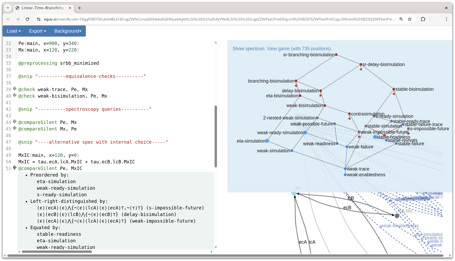
@compareSilent Pe, MxICPe aligns much better to the MxIC-specification! “@compareSilent Pe, MxIC” returns:
• Preordered by:
    eta-simulation
    weak-ready-simulation
    s-ready-simulation
• Left-right-distinguished by:
    ⟨ϵ⟩⟨ecA⟩⟨ϵ⟩Λ{¬⟨ϵ⟩⟨lcA⟩⟨ϵ⟩⟨ecA⟩⊤,¬⟨τ⟩⊤} (s-impossible-future)
    ⟨ϵ⟩⟨ecB⟩⟨ϵ⟩⟨lcB⟩Λ{¬⟨ϵ⟩⟨ecB⟩⊤} (delay-bisimulation)
    ⟨ϵ⟩⟨ecA⟩⟨ϵ⟩Λ{¬⟨ϵ⟩⟨lcA⟩⟨ϵ⟩⟨ecA⟩⊤} (weak-impossible-future)
• Equated by:
    stable-readiness
    eta-simulation
    weak-ready-simulation
The output means that implementation Pe and internal choice specification MxIC cannot be distinguished from each other by a readiness observation (subsuming failures), neither in stable nor weak semantics. Interestingly, in weak (that is, unstable) semantics the indistinguishability goes even further, up to weak ready simulation.
The tool’s visual output of the spectrum for Pe vs. MxIC (Figure 8.2) also sports a bigger blue region of equivalence than with the original specification (cf. Figure 1.3).
The main aspect that creates the differences between Pe and MxIC is that the implementation can decide that B will be the next entering the critical section next, even before A has left. In above output, this is mirrored by the impossible-future formula ⟨ϵ⟩⟨ecA⟩⟨ϵ⟩Λ{¬⟨ϵ⟩⟨lcA⟩⟨ϵ⟩⟨ecA⟩⊤}.
We can find this scenario already in the pseudocode. It happens when both processes are in PC = 2 and B has set turn = A. Then, A may enter its critical section but has to yield to B before it can re-enter. So, this constitutes a proper difference between Peterson’s protocol and a pure iterated internal choice. But then again, one might say that it is fair of the process going first to leave the next round to the other waiting participant. In the pure CCS view, however, we cannot adequately treat more general fairness considerations for Peterson’s protocol, as van Glabbeek (2023) explicates.
This is what the spectroscopy has taught us: Peterson’s mutual exclusion protocol is more similar to repeated internal choice (MxIC) than to the specification Mx from Aceto et al. (2007). However, the two are not bisimilar in any sense, since, in Pe, local progress from one iteration may influence the next.
8.1.3 Program Structure
The core of equiv.io aligns quite closely to the spectroscopy framework outlined in Figure 5.1. In this subsection, we take a quick look at how implementation and definitions in this thesis correlate.

Figure 8.3 shows core transformations that happen in the process of analyzing the equivalences for a pair of processes:
Parsing.
 ccs.Parser transforms source into an abstract syntax tree object
 ccs.Syntax.Definition, along the lines of Definition 2.2 with the syntax of Section 8.1.1.Interpretation.
ccs.Interpreter applies the operational semantics of Definition 2.31 to construct a ts.WeakTransitionSystem, which supports silent-step transitions of Section 6.1.1. Also the preprocessing of Section 8.1.1 is applied, the soundness of which follows Lemma 5.4 (and its analogues for the weak spectrum).Spectroscopy. The trait
spectroscopy.SpectroscopyFramework orchestrates the spectroscopy pipeline. Its abstract parts are instantiated by spectroscopy.StrongSpectroscopy and spectroscopy.WeakSpectroscopy for the respective spectroscopy variants of Chapter 5 and Chapter 7. In particular, they facilitate the following steps in SpectroscopyFramework.decideAll:- The spectroscopy implementation defines a spectroscopy game (e.g. spectroscopy.StrongSpectroscopyGame). The game must be a game.EnergyGame, inheriting a decision procedure along the lines of Algorithm 4.1 from trait game.GameLazyDecision. This computation is invoked together with the game graph construction through
populateGame. - The spectroscopy provides an hml.Spectrum object which is used to interpret the game result in a hierarchy of hml.ObservationNotions to pick the strongest preorders to relate compared processes. The specifics of Chapter 3 and Chapter 6 are implemented by hml.StrongObservationNotion and hml.WeakObservationNotion.
- The spectroscopy implements a
buildHMLWitness-method, constructing strategy formulas from attacker-won budgets of \mathsf{Strat}_{\triangle} in Definition 5.2 and \mathsf{Strat}_{\nabla} in Definition 7.2.
- The spectroscopy implementation defines a spectroscopy game (e.g.
Validation (optional). If the user demands,
SpectroscopyFramework.decideAllcontinues to construct cheapest distinguishing formulas for the query withbuildHMLWitness.- hml.Interpreter checks that each formula is indeed true for one process and false for the other, applying the semantic HML game of Section 2.4.2. If the formula is not distinguishing, an exception is thrown.
classifyFormulaon the specificSpectrumobject determines the expressiveness prices of formulas (implemented as in Remark 3.1 and Definition 6.11 by theformulaObsNotionfunctions inhml.StrongObservationNotion / hml.WeakObservationNotion). If the formula price exceeds the budget predicted by the game or is unexpectedly cheap, this constitutes an error.
Error reports would point to incorrectness of the specific spectroscopy, not to user mistakes. Thus, the validation does not affect the core decision procedure, but increases confidence that a specific output is sound.
If no formula construction is requested,
SpectroscopyFramework.decideAllworks on flattened energies (Definition 4.13), which generally leads to better performance.Presentation.
SpectroscopyFramework.decideAllcollects the finest preorders and coarsest distinctions, optionally together with their witness formulas in aSpectroscopy.Resultobject fromspectroscopy.Spectroscopy. This object helps front-end layers of the tool interpret the output as spectra, equivalences, and distinguishing formulas.
1 There is a minor semantical difference: The equiv.io interpreter flattens process restriction in recursion. This leads to processes like P = a.P \ {b} having a finite process graph instead of an infinite one (cf. Aceto et al., 2007, Exercise 2.9).
Another trait spectroscopy.EquivalenceChecking follows the second path of Figure 5.1 to decide individual equivalences through reachability games. We will not go into detail here. The core feature is to derive a game game.MaterializedEnergyGame as in Definition 4.4. game.WinningRegionComputation determines its winner according to Algorithm 2.1.
Besides the core-flow, there are some small additional diagnostic features. For instance, spectroscopy.SpectroscopyFramework can save the spectroscopy game graph and formulas in Graphviz-format using game.GameGraphVisualizer, comparable to Figure 4.7. The output of the same mechanism for spectroscopy.EquivalenceChecking appears, for example, in the derived trace game of Figure 5.7.
Remark 8.1 (Line counting). When following the links to source listings above, you might notice that most aspects only take a few hundred lines of code. Depending on how one counts, a total of 2000–3000 lines fit the two spectroscopies, preorder checking for all the notions, game algorithms, generation and validation of HML formulas, and presentation mechanisms.
As far as code bases go, that size is extremely compact.2 In part, this is enabled by Scala’s conciseness. But the heavy lifting in making the implementation so light-weight is achieved by the energy-game abstraction.
2 For reference, Cleaveland & Sims (1996) report 18,000 LOC for the NSCU Concurrency Workbench in Standard ML. Performance-centric C++ code bases like mCRL2 (Bunte et al., 2019; Groote & Mousavi, 2014) are another order of magnitude bigger.
Remark 8.2 (Tests). The codebase of the backend of equiv.io includes test suites for strong and weak spectroscopy. These ensure that the algorithms (with and without optimizations) return the expected results for the finitary separating examples of strong and weak spectrum (van Glabbeek, 1990, 1993). This provides some confidence that not too much is going astray on the way between our correctness theorems and optimized implementation.
8.1.4 Benchmarks
Our algorithm and equiv.io are aimed at small transition systems that “fit onto one screen.” But still, the backend can analyze the equivalence structure of moderately-sized real-world transition systems. In this subsection, we examine its performance on the VLTS (“very large transition systems”) benchmark suite Garavel (2017) and on our recurring Peterson example.
Clever strong spectroscopy. Table 8.3 reports the results of running the backend with the clever strong spectroscopy game \mathcal{G}_{\blacktriangle}. This mostly matches the results already reported in Bisping (2023b).3
3 The benchmarking is in the class tool.benchmark.VeryLargeTransitionSystems. It can be started via sbt "shared/run benchmark --strong-game --reduced-sizes --include-hard".
The benchmark uses the VLTS examples of up to 25,000 states and the Peterson example. The table lists the \mathcal{P}-sizes of the input transition systems and of their strong bisimilarity quotient system {\mathcal{P} \! / \!\! \sim_\mathrm{B}} (Definition 2.10).
The test suite constructs the game graph on the quotient system, starting at all positions that compare pairs of enabledness-equivalent states. The \mathrel{\smash{›\!\!\frac{\scriptstyle{\;\enspace\;}}{}\!\!›}}_\blacktriangle-column reports the size of the discovered game graph in terms of moves. The time-column lists execution times of the spectroscopy procedure in seconds.4
4 Average of mid three runs out of five, in the Java Virtual Machine with 8 GB heap space, single-threaded on Intel® Core™ Ultra 7 155H.
The last three columns list the output sizes of state spaces reduced with respect to enabledness \mathrm{E}, traces \mathrm{T}, and simulation \mathrm{1S}.
From the output, we learn that the VLTS examples, in a way, lack diversity: Bisimilarity \mathrm{B} and trace equivalence \mathrm{T} coincide on the systems (third and penultimate column).
Concerning the algorithm itself, the experiments reveal that the computation time grows mostly linearly with the size of the game move graph. On vasy_18_73, the implementation times out after 500 seconds.
Of those terminating, the heavily nondeterministic cwi_1_2 is the most expensive example. Almost all of its transitions are labeled by i, standing for internal activity \tau in the VLTS suite. As many coarse notions must record the nondeterministic options, this blow-up is to be expected. If we compare to the best similarity algorithm by Ranzato & Tapparo (2010), they report their algorithm SA to tackle cwi_1_2 single-handedly. Like our implementation, the prototype of SA of Ranzato & Tapparo (2010) ran out of memory while determining similarity for vasy_18_73. This is in spite of SA theoretically having optimal complexity and similarity being less complex than trace equivalence, which we need to cover (cf. Section 3.3.3). The benchmarks in Ranzato & Tapparo (2010) failed at vasy_10_56, and vasy_25_25, which might be due to 2010’s tighter memory requirements (they used 2 GB of RAM) or the degree to which bisimilarity and enabledness in the models is exploited.
Simplified weak spectroscopy. Table 8.4 lists analogous values for the weak spectroscopy game \mathcal{G}_{\widehat{\nabla}}, in the simplified variant, but also containing revivals moves of Section 7.3.2.
| System | \mathcal{P} | {\mathcal{P} \! / \!\! \sim_\mathrm{BB^{sr}}} | \mathrel{\smash{›\!\!\frac{\scriptstyle{\;\enspace\;}}{}\!\!›}}_{\widehat{\nabla}} | time (s) | {\mathcal{P} \! / \!\! \sim_\mathrm{WE}} | {\mathcal{P} \! / \!\! \sim_\mathrm{WT}} | {\mathcal{P} \! / \!\! \sim_\mathrm{1WS}} |
|---|---|---|---|---|---|---|---|
peterson |
36 | 21 | 3,579 | 0.10 | 5 | 16 | 16 |
vasy_0_1 |
289 | 9 | 2,958 | 0.07 | 3 | 9 | 9 |
cwi_1_2 |
1,952 | 67 | 22,944 | 0.40 | 19 | 67 | 67 |
vasy_1_4 |
1,183 | 4 | 0 | 0.00 | 4 | 4 | 4 |
cwi_3_14 |
3,996 | 2 | 0 | 0.00 | 2 | 2 | 2 |
vasy_5_9 |
5,486 | 112 | 2,723 | 0.06 | 91 | 112 | 112 |
vasy_8_24 |
8,879 | 170 | 10,983 | 0.12 | 115 | 169 | 169 |
vasy_8_38 |
8,921 | 193 | 32,598 | 0.35 | 104 | 193 | 193 |
vasy_10_56 |
10,849 | 2,112 | - | - | - | - | - |
vasy_18_73 |
18,746 | 2,326 | - | - | - | - | - |
vasy_25_25 |
25,217 | 25,217 | 0 | 0.32 | 25,217 | 25,217 | 25,217 |
The algorithmic setup is slightly changed for the weak setting: We work with the quotient system of stability-respecting branching bisimilarity and start at weakly enabledness-equivalent pairs. The last three columns give the output quotient sizes for weak enabledness \mathrm{WE}, weak traces \mathrm{WT}, and weak simulation \mathrm{1WS}.
The peterson example, after minimization, has exactly the 21 states shown in Figure 1.2. Its weak similarity quotient is smaller (16 states, cf. last column), which fits our observations that weak similarity equates more in this model than bisimilarity-like notions do.5
In weak semantics, cwi_1_2 becomes easy, as its internal nondeterminism is directly compressed away by the initial branching-bisimilarity minimization.
Again, we see that branching bisimilarity and weak trace equivalence mostly coincide on the VLTS examples. Only vasy_8_24 differs between 170 states in {\mathcal{P} \! / \!\! \sim_\mathrm{BB^{sr}}} and 169 in {\mathcal{P} \! / \!\! \sim_\mathrm{WT}}.
The numbers align with the output of a different implementation in Bisping & Nestmann (2019), which is a good sign for the correctness of both programs. There, the same samples were analyzed with respect to coupled similarity, a weak notion close to contrasimilarity and weak similarity. Interestingly, the coupled simulation implementation in Bisping & Nestmann (2019) takes minutes for vasy_25_25, constructing a game with 126,000 moves. The trivial game of Table 8.4 suggests that this would not be necessary.
In summary, the equivalences of our spectra mostly coincide on the considered VLTS samples. This indicates that the examples are based around models that avoid the expressive power of finer branching-time notions.
8.2 Student Implementations
There exist three other implementations of the equivalence spectroscopy algorithm by students of mine. Each covers a different direction: In Section 8.2.1, we discuss The Spectroscopy Invaders, a computer-game version, which has an educational purpose. Section 8.2.2 presents an extension to an existing educational tool, the Concurrency Workbench Aalborg Edition. Section 8.2.3 closes by reporting on gpuequiv, a performance-centric shader-based implementation using the modern WebGPU standard.
8.2.1 Computer Game: The Spectroscopy Invaders
Would it not be nice if one could play the spectroscopy game as a game?
Trzeciakiewicz (2021) develops the computer game “The Spectroscopy Invaders” where one plays the attacker in the spectroscopy game. You can enjoy the game in the browser at https://games.equiv.io/play/ltbt-game/.
A play of the game corresponds to naming a universal attack strategy in the strong spectroscopy game of Definition 5.1, or, equivalently, to constructing a distinguishing formula. To reach maximal level scores, one has to play out a minimal formula in the sense of our pricing. Under the hood, the TypeScript implementation uses Bisping et al.’s (2022) algorithm to compute the minimal budgets. The game does not present the costs of moves to the player, but they matter for the scores received at the end of a level.
Figure 8.4 gives a screenshot of the first level of the “Failure” world.6 This level corresponds to the classic Example 2.1 of \mathsf{P} and \mathsf{Q} if we match the orange transitions to \tau-steps, blue to \mathsf{a}, and yellow to \mathsf{b}. The metaphor on top of the game mechanics is that the human-controlled hero (left) has to outmaneuver a group of elves (right) that might split up on nondeterministic transitions.
6 In the online version of this thesis, it is actually a screen capture by Trzeciakiewicz, illustrating negation moves in the game tutorial.
From Example 5.3, we know that the failure \langle \tau \rangle\neg\langle \mathsf{a} \rangle is a cheapest distinction of the left state from the right in this system, translated as \langle \mathsf{orange} \rangle\neg\langle \mathsf{blue} \rangle. In the computer game, we would use this distinction as follows: First click on the state behind the middle orange transition to observe it. Then, click on the “negation” button  to swap sides of hero and elve. Defeat them by moving along the right blue edge.
The handling of conjunctions is a little more involved.

Figure 8.5 shows the second level of the “Simulation” world. In the level, the player’s task is to distinguish \mathsf{white}\ldotp\!(\mathsf{red} +\mathsf{orange}\ldotp\!\mathsf{orange}) (left) from \mathsf{white}\ldotp\!(\mathsf{red}+\mathsf{orange}) +\mathsf{white}\ldotp\!\mathsf{orange}\ldotp\!\mathsf{orange} (right). The current game position occurs after the first white observation and corresponds to \smash{\color{gray}[}\mathsf{red} +\mathsf{orange}\ldotp\!\mathsf{orange}, \{\mathsf{red}+\mathsf{orange}, \mathsf{orange}\ldotp\!\mathsf{orange}\}\smash{{\color{gray}]}_\mathtt{a}^{\color{gray} \scriptscriptstyle}} in the strong spectroscopy game \mathcal{G}_{\triangle}, as indicated by the hero figure on the left and the two elves on the right.
The player can click the “conjunct” button  , after which they have to explain how to win \smash{\color{gray}[}\mathsf{red} +\mathsf{orange}\ldotp\!\mathsf{orange}, \mathsf{red}+\mathsf{orange}\smash{{\color{gray}]}_\mathtt{a}^{\color{gray} \scriptscriptstyle\land}} and then \smash{\color{gray}[}\mathsf{red} +\mathsf{orange}\ldotp\!\mathsf{orange}, \mathsf{orange}\ldotp\!\mathsf{orange}\smash{{\color{gray}]}_\mathtt{a}^{\color{gray} \scriptscriptstyle\land}}. In the split state, the player can first click through the yellow-arrow successor states on the left to point out that the left elve cannot observe two yellow steps. Then, they also have to name how to defeat the right elve, by taking the red transition. Together, this strategy corresponds to the simulation formula \textstyle\bigwedge \{\langle \mathsf{yellow} \rangle\langle \mathsf{yellow} \rangle, \langle \mathsf{red} \rangle\}.
The game is single-player, also in a theoretical sense: There is no picking of conjunction answers by the defender. Instead, the attacker has to name attacks for every right-hand state. Due to nested conjunctions, the game positions thus actually are sets of \smash{\color{gray}[}p, Q\smash{{\color{gray}]}_\mathtt{a}^{\color{gray} \scriptscriptstyle}} tuples.
Trzeciakiewicz (2021) limits the scope to (strong) trace, failure, possible-future, simulation, and bisimulation equivalences, excluding notions like readiness, ready traces, and failure traces. The selection permits slightly simpler game rules—in particular, without revival moves. This allows to nicely showcase the core mechanics of Chapter 5 with a stricter correspondence to productions in the original HML of Definition 2.11.
8.2.2 CAAL Extension
Would it not be nice if one could use the equivalence spectroscopy in existing tools?
Ozegowski (2023) integrates the spectroscopy algorithm into CAAL, the “Concurrency Workbench Aalborg Edition” by Andersen et al. (2015). Straßnick & Ozegowski (2024) also add the weak spectroscopy game and possibilities to play the spectroscopy game in the tool. Their extended version of CAAL is live on https://equivio.github.io/CAAL/.
The original CAAL (on https://caal.cs.aau.dk/) covers the curriculum of Reactive systems (Aceto et al., 2007), including CCS processes, HML formulas and equivalence games.
Originally, CAAL only supports preorder/equivalence checking for six standard notions, namely for simulation, bisimulation, and traces, in their standard strong and weak variants. Only simulation and bisimulation can be examined as games.
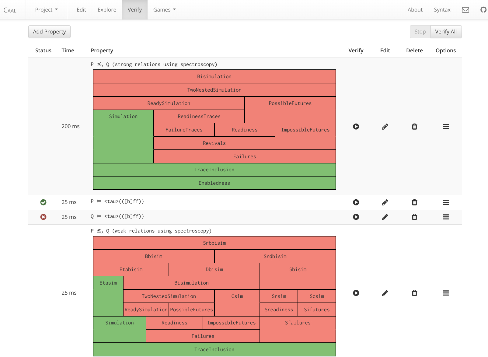
Straßnick and Ozegowski’s extended CAAL version supports 13 strong and 21 weak notions. Each of the notions can be decided individually, or in the context of a spectroscopy. For the strong notions, the game graph can be explored interactively. Figure 8.6 shows the output of strong and weak spectroscopy on the classic Example 2.1, together with a generated distinguishing failure formula in the HML dialect of CAAL.
For a usage guide, we refer to Straßnick & Ozegowski (2024).
At some points, Straßnick and Ozegowski’s fork unfortunately has to remain partial with respect to features. For instance, the extension does not support distinguishing formulas for the weak spectroscopy because CAAL’s HML dialect cannot easily be molded to support \mathsf{HML}_{\mathsf{SRBB}}.
Still, the project shows that the spectroscopy approach is sufficiently simple and versatile to allow dozens of equivalence checkers to be integrated into existing tools within the limited scope of a student project.
8.2.3 GPU Implementation: gpuequiv
Would it not be nice if one could use modern hardware to perform spectroscopies as fast as possible?
Vogel (2024) implements the strong equivalence spectroscopy in gpuequiv using shaders in the WebGPU Shading Language (Baker et al., 2025).
Technically, this is superior to the other three implementations of this chapter, which can only exploit the single-threaded CPU model of JavaScript when running in the browser.
Historically, the WebGL standard for browser graphics processing has lacked compute shaders. This has made it difficult to access the computational power of graphics processing units from within web applications. Times are changing with WebGPU/WGSL (Baker et al., 2025). Vogel (2024) makes this technological progress available to the spectroscopy approach.
Big parts of the game graph construction and the game solving are quite parallelizable. gpuequiv parallelizes the budget computation of Algorithm 4.1. For instance, a whole batch of game positions on a todo-list can be processed simultaneously. The details are explained by Vogel (2024).
gpuequiv’s control code surrounding the shader invocations is written in Rust that can be compiled to native code and to WebAssembly. Therefore, gpuequiv can be compiled for both kinds of targets: Quick equivalence checking in the browser, and even quicker checking in a native application. Vogel (2024) reports 10⨯ speed-ups compared to Bisping (2023b). However, the fast growth of game graphs remains a limiting factor as larger examples run into the size boundary of buffers to upload game moves. For the system vasy_18_73, Vogel (2024) also fails to complete the spectroscopy (like our experience in Section 8.1.4): It constructs a game graph of 623,482,227 moves, but only 536,870,911 moves fit into the buffer with the employed data packing.
At the time of writing, another Bachelor project is underway to add a frontend and support for the weak spectroscopy game to gpuequiv.
8.3 Discussion
In this chapter, we have surveyed the four existing implementations of the spectroscopy algorithm.
We focused on equiv.io, which closely aligns with this thesis. We have seen how the tool easily answers questions such as “How equivalent is Peterson’s algorithm to the specification of mutual exclusion.” equiv.io can check behavioral preorders and equivalences for more than 39 notions of strong and weak spectrum. Due to the possibility to mark divergences, even more notions are available via preprocessing.
Other tools. A recent survey by Garavel & Lang (2022) lists hundreds of tools to check bisimilarity and related equivalences and preorders. Some of them can justify their output with distinguishing formulas (or traces), similar to our approach. Many specific tools address special equivalences, for instance for open, timed, or probabilistic systems, which we do not support. On the other hand, equiv.io might be the first tool to cover some of the more arcane notions of the weak spectrum (van Glabbeek, 1993), such as \eta-similarity and stable bisimilarity.
In Table 8.5, we compare the supported notions of equiv.io to four current state-of-the-art tools. A tick ✔ stands for direct support, (✔) for support via preprocessing.
| Equivalence / preorder | equiv.io | CAAL | mCRL2 | CADP | FDR4 |
|---|---|---|---|---|---|
| Strong / weak enabledness | ✔ | ||||
| Strong trace | ✔ | ✔ | ✔ | ✔ | |
| Weak trace | ✔ | ✔ | ✔ | ✔ | ✔ |
| Strong failure | ✔ | ✔ | |||
| Weak failure | ✔ | ||||
| Stable failure | ✔ | ✔ | ✔ | ||
| Failure-divergence | (✔) | ✔ | ✔ | ||
| Strong / stable revivals | ✔ | ||||
| Strong / weak / stable readiness | ✔ | ||||
| Strong / stable failure-trace | ✔ | ||||
| Strong / stable ready-trace | ✔ | ||||
| Strong / stable impossible fut. | ✔ | ||||
| Weak impossible future | ✔ | ✔ | |||
| Strong / weak possible future | ✔ | ||||
| Strong simulation | ✔ | ✔ | ✔ | ||
| Weak simulation | ✔ | ✔ | |||
| Stable simulation | ✔ | ||||
| \eta-simulation | ✔ | ||||
| Safety / \tau^*.a | ✔ | ||||
| Strong ready-simulation | ✔ | ✔ | |||
| Weak / stable ready-simulation | ✔ | ||||
| 2-nested strong / weak sim. | ✔ | ||||
| Strong bisimulation | ✔ | ✔ | ✔ | ✔ | (✔) |
| Contrasim. / stable bisim. | ✔ | ||||
| Coupled simulation | ✔ | ||||
| Weak bisimulation | ✔ | ✔ | ✔ | ✔ | (✔) |
| Div.-pr. weak bisim. | (✔) | ✔ | (✔) | ||
| Delay bisimulation | ✔ | (✔) | |||
| Stability-resp. delay bisim. | ✔ | ||||
| \eta-bisimulation | ✔ | ||||
| Branching bisimulation | ✔ | ✔ | ✔ | ||
| Stability-resp. branch. bisim. | ✔ | ||||
| Div.-pr. branching bisim. | (✔) | ✔ | (✔) |
- CAAL (Andersen, Andersen, et al., 2015), or the “Concurrency Workbench Aalborg Edition,” also works with CCS and has already been discussed in Section 8.2.2.7
- mCRL2 (Groote & Mousavi, 2014), built around an ACP/CCS-like modelling language of the same name, supports a wide-range of notions with highly efficient implementations and a strong focus on branching bisimilarity. On the notions that it supports, it will generally be much faster than the spectroscopy game algorithm. The only notion that is exclusively supported by mCRL2 is coupled similarity, implemented by Lê (2020).
- CADP (Garavel et al., 2013) can check several notions on-the-fly, also in a highly optimized fashion. Its models are usually expressed in LOTOS or LNT, deriving from CSP. It includes the special notions of safety- and \tau^*\!.a-equivalence, not present in van Glabbeek’s spectrum (1993).
- FDR4 (Gibson-Robinson et al., 2014) has “Failures Divergences Refinement” in its name, but also supports different linear-time refinement models for CSP. Branching-time notions are partially supported as minimizers.
7 Andersen, Hansen, et al. (2015, Section 3.3) also mention how to use their game backend to handle 2-nested simulation and ready-traces. But this is neither elaborated upon nor supported in the frontend.
Like the listed tools, equiv.io can be seen as following the tradition of the discontinued “Concurrency Workbench[es]” (Cleaveland et al., 1990; Cleaveland & Sims, 1996).
Other avenues for implementation. The implementations of this chapter realize Algorithm 4.1 quite directly to decide energy games. Among them, the shader version of Section 8.2.3 adds the highest level of implementation cleverness with respect to packing of data and parallelization of computation. But so far, we are not using the full toolbox of the computer-aided-verification community.
For instance, the upward-closed sets of winning budgets could be handled more symbolically with the representation of Delzanno & Raskin (2000). This might slightly increase how many Pareto fronts can be kept in memory. But one can expect that its payoff would be meager, especially on the small \{0,1,\infty\}^d-lattices. Experiments by Vogel (2024) suggest that the Pareto fronts usually stay sufficiently small that adding the implementation complexity of Delzanno & Raskin (2000) seems uncalled for.
A big limiting factor of our implementations is the storage of the game graph. To some extent, this can be battled by more symbolic representations as binary-decision-diagrams. Bulychev (2011) and Wimmer (2011) follow this route in quite versatile checkers.
A more general solution for the memory limitations would be to forget parts that have been visited, and recompute them by-need. There are easy ways to profit from the community’s advances in handling big spaces of possibilities. The most prominent would be to instantiate the game rules for a transition system, and feed them into an SMT solver. Already Shukla et al. (1996) suggest a comparable approach, viewing games as SAT problems. The energy aspect should be perfectly expressible for SMT/SAT solvers in linear integer arithmetic (cf. Chistikov, 2024).
Alternative paths to generalized checkers. In Section 2.5, we have already discussed the alternative paradigms of equivalence checking. The equivalences-as-game-instances approach seems to be the most fruitful when one wants to easily support a wide range of preorders and equivalences in a tool. By “easy,” we mean: without the need to implement individual algorithms for each of the notions. Tan (2002) takes a similar game approach for the Concurrency Workbench, as do Andersen, Hansen, et al. (2015) for CAAL.
Another route to this goal of genericity might be the approach of equivalences-as-formulas from Lange et al. (2014). The idea there is to use a diadic higher-order \mu-calculus where one can talk about relations between states. Thereby, the rules of how to preorder states can be expressed as formulas. One only needs to implement the model-checking for formulas once, and new notions could be added by only adding new formulas. Stöcker (2024) implements this idea successfully. But the data suggests that 20 states already demand several seconds in this approach for some equivalences.
The third path to genericity is through equivalences-as-functors, to enable coalgebraic partition-refinement algorithms from category theory. We already hinted to this in Section 2.5. Deifel et al. (2019) follow this route in their tool CoPaR (short for “Coalgebraic Partition Refiner”). This way, the support of new equivalences boils down to a few lines of defining new functors. The big advantage is that extensions—for instance, to quantitative behavioral distances—can also be achieved this way. The coalgebraic approach is related to the game approach and, too, can derive distinguishing formulas, as seen for instance in the tool T-BEG (König et al., 2020). However, encoding simulation-like preorders in category theory seems to be non-trivial if one compares the machinery of Ranzato & Tapparo (2010) to the ease of just leaving out swap-moves in the bisimulation game. It is difficult to say whether it is conceptional boundaries or the coating in category-theory parlance that has hindered a wider adoption in tools.
A light-weight variant of the functor-approach is offered by the paradigm equivalences-as-signatures. Tools like Sigref (Wimmer et al., 2006) support a broad range of bisimulation-like equivalences. The specifics of individual equivalences are expressed as signatures that prescribe how to refine equivalence classes in an iterative partition-refinement. Signature Refinement can easily be boosted by parallelization or symbolic BDD-encodings.
Of course, all these theoretical approaches are linked on some basic level, namely through the Hennessy–Milner theorem (Theorem 2.1). We elaborate on this in the conclusion.